Happy #RealTimeChem week everybody.  What, you don’t know what it is?  Neither did I, untill I happened to read about it over at Compound Interest . (You guessed it, I’ve got lots of grading to do so I’m procrastinating again.) Since the theme this year centers on the four new elements that have been added to the periodic table, and I have an affinity for the table and all its secrets, I thought it might be fun to take advantage of the periodic properties of the table and predict some of the characteristics of the new elements.

I’m going to use Mathematica to help with this project for several reasons.  First, (and perhaps foremost) I’m familiar with the language.  Second, it has a lot of curated data sets, one of which is ElementData that contains useful information for this project.  Third, my approach is going to be very visual, and having a single system for accessing, manipulating and visualizing data makes Mathematica useful for this project.  Plus, umm, I’m familiar with the language.

I’ll start off with this guiding question: What are the atomic radii of the period 7 p block elements? First, let’s get an overview of what the periodic trend in atomic radii looks like.

(* To make curated data queries a bit easier to handle *)
SetSystemOptions[SystemOptions["DataOptions"] /. True -> False];
(* Get the table *)
Rasterize[
 WolframAlpha[
  "periodic table", {{"PeriodicTableProperties:ElementData", 1}, 
   "Content"}, 
  PodStates -> {"PeriodicTableProperties:ElementData__Atomic \
radius"}], ImageSize -> 600]

Wolfram alpha has a nice enough periodic table that allows me to display the atomic radius along with the elemental symbol.  Note that the curated dataset is not quite up to date with the period 7 names yet.

allelements = 
  DeleteCases[
   Outer[ElementData, Range[118], {"AtomicNumber", "AtomicRadius"}], 
   x_ /; MemberQ[Head /@ x, Missing]];
ListPlot[allelements, Filling -> Axis, 
 Frame -> {True, True, False, False}, 
 FrameLabel -> {"Atomic Number", "Atomic Radius (pm)"}, 
 FillingStyle -> LightBlue, PlotStyle -> Red, AspectRatio -> 0.5]

When atomic radius is plotted as a function of atomic number, two trends emerge.  The most shocking is that there are series of decreases in atomic radius as the atomic number gets larger.  Each one of these series starts a little bit higher than the previous one, so there is a general increase in radius.  For the uninitiated, this pattern is unexpected, since it makes more sense to think that the size would continue to increase since the atomic weight continues to increase.  The reason (short answer) for this behavior is effective nuclear charge, which I won’t say more about in this discussion.

Let’s focus in on the p-block

(* Get pblock data, remove entries with missing information *)
pblockdata = DeleteCases[
   Outer[ElementData, 
    ElementData["PBlock"], {"AtomicNumber", "Period", "Group", 
     "AtomicRadius"}],
   x_ /; MemberQ[Head /@ x, Missing]
   ];

(* Plot data as a bar chart and make it pretty *)
BarChart[Table[
  Labeled[Last /@ GroupBy[pblockdata, #[[3]] &][i], 
   "Group\n" <> ToString@i], {i, 13, 18}], 
 AxesLabel -> {None, "Radius (pm)"}, 
 ChartLegends -> ("Period " <> ToString@# & /@ Range[2, 6])]

In this slightly non-conventional view, we see again that the atomic radius increases within a group as the period increases and that for a given period, the radius decreases with increasing group.  Looking closely at periods greater than 2, the trend with increasing group number seems remarkably linear:

(* Quick and dirty plot of p-block radii trends *)
With [{d = GroupBy[Select[pblockdata, 3 <= #[[2]] <= 6 &], #[[2]] &]},
  Table[d[i][[All, {1, 4}]], {i, Keys[d]}]
  ] // ListPlot

The linearity allows me to create a best fit line that would predict the radius if I know the period.  I wonder if there is a relationship between the slopes and intercepts of these best-fit lines so that I could create a function that generates a radius estimate given the atomic number, group and period.

lm = LinearModelFit[#, {x, 1}, x] & /@ 
   With [{d = 
      GroupBy[Select[pblockdata, 3 <= #[[2]] <= 6 &], #[[2]] &]},
    Table[d[i][[All, {1, 4}]], {i, Keys[d]}]
    ];
TableForm[#["BestFitParameters"] & /@ lm, 
 TableHeadings -> {("Period " <> ToString@# & /@ 
     Range[3, 6]), {"slope", "intercept"}}]

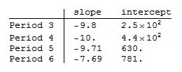
First, I see that the slopes cluster around -9.8 pm/Z except for period 6, which is quite different.  I’m going to hazard a guess that the lanthanide contraction is playing a role here, and the difference is due to the way f-orbitals behave.  The differences in intercepts fall nicely on a straight line.

With[{d = 
   Transpose[{{3, 4, 5, 6}, #["BestFitParameters"][[2]] & /@ lm}]},
 blm = LinearModelFit[d, {x, 1}, x];
 Plot[blm[x], {x, 2, 7}, Epilog -> {PointSize[0.02], Point /@ d}, 
  Frame -> {True, True, False, False}, 
  FrameLabel -> {"Period", "intercept of\nradius fit"}]
 ]

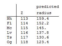
We can get the intercept for period 7 easily with N@blm[7] which returns 973 pm.  Now I think we have enough information to make a model.  I am going to assume that the p-block period 7 elements follow a linear trend in atomic radii.  Based on the trends for periods 3 through 6, I predict that the intercept for this linear model is 973.  The slope is a bit tricker and requires some fudge-work.  I suspect it will be close to -7.6 because of the presence of f-orbitals.  I also believe it will be a little bit lower, but by how much?  I’m going to make a non-educated guess and say that the slope would decrease by about 5%, which gives me radius = -7.2 Z + 973 as the function for estimating the radii of period 7 p-block elements.

p7[z_] := -7.2 z + 973
TableForm[Table[{z, p7[z]}, {z, 113, 118}],
 TableHeadings -> {{"Nh", "Fl", "Mc", "Lv", "Ts", "Og"}, {"\nZ", 
    "predicted\nradius"}}]

BarChart[
 With[{
   a = Table[Last /@ GroupBy[pblockdata, #[[3]] &][i], {i, 13, 18}],
   b = Table[p7[z], {z, 113, 118}]
   },
  MapThread[Join[#1, {#2}] &, {a, b}]
  ],
 AxesLabel -> {None, "Radius (pm)"}, 
 ChartLegends -> ("Period " <> ToString@# & /@ Range[2, 7])]

The prediction doesn’t look totally unreasonable.  There is a little surprise in my prediction, and that is the radius of flevorium may be smaller than the atomic radius of lead.  Given that we have no reasonable estimates of atomic radii for the actinoids (that I’m aware of), I suspect it will be quite some time before we get a more sophisticated estimate of the radii.

One last comment.  Recent versions of Mathematica have incorporated neural networking into the software package, which makes me wonder if I could do all of this in a much easier fashion.

pf = Predict[pblockdata[[All, {1, 2, 3}]] -> pblockdata[[All, 4]]];

TableForm[Table[{z, p7[z], pf[{z, 7, z - 100}]}, {z, 113, 118}],
 TableHeadings -> {{"Nh", "Fl", "Mc", "Lv", "Ts", "Og"}, {"Z", 
    "linear", "neural"}}]

Hmm, the two models agree reasonably well, and the neural network blows my Fl vs. Pb prediction out of the water.  Not sure what to make of that, except that there does seem to be value in exploring the periodic properties of the elements.

In conclusion, not that I’m intentionally advertising for Wolfram here, but the ability to access data, manipulate it and visualize the results with a single platform made this project fairly tractable.  The periodic table holds many secrets worthy of exploration, and the trends in physical and chemical characteristics are not only useful in finding structure/function relationships, but also to predict the properties of new elements.  Given that the father of the periodic table is known for his predictions makes this last point not all that surprising.  I find it quite exciting that we can still engage in predictive model making so many years after the table was first proposed.