
This is the first of a new series (tag) Dancing with Wolfram. Occasionally, I need to work through programming strategies in Wolfram, and I need a place to store my ideas. Perhaps they will be useful to others.
The problem
When collecting data from a sensor, one wants to generate a list of {x, y} pairs where x is typically time and y is the sensor reading. One way of doing this is to create an empty list and then using Mathematica’s AppendTo function to add elements to the list. The problem with this approach, however, is that it is not very efficient. The function call makes a copy of the original list each time, and when the list of data gets very large, the time it takes to store a data point increases. Below, I’ve plotted the average time needed to store a datapoint as a function of the list size. For comparison, I’ve collected data (times measured on a Raspberry Pi v2) using AppendTo with a list (blue dots) and adding key -> value pairs to an association (orange dots).
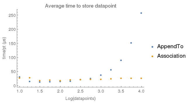
After about 1000 data points, the AppendTo a list approach starts to take increasingly longer times. I was unable to collect any data beyond 10,000 data points since AppendTo started running into memory issues. It is not unreasonable to expect a sensor data set to contain in excess of 1000 data points, so the performance of AppendTo is not acceptable.
Introducing Associations
In version 10 of Mathematica, Wolfram introduced a new type called Association. An association stores information in a key -> value pair and as the figure above shows, adding elements to an Association doesn’t run in to the same problems as a list. Using an Association does generate some additional complexity when it comes time to visualize the data. Presently, I’m thinking of two different methods for storing data points in an Association:
- Using an arbitrary, incremental key with the value being the data point (# -> {x,y})
- Using the key as the abscissa and the value as the ordinate (x -> y)
My task now is to determine which method is more efficient. I’m defining efficiency using the following criteria
- Time needed to store a data point (shorter is better)
- Complexity of code needed to transform data into a list (readable and fast)
- Memory used for data storage (less is better)
Method 1: # -> {x,y}
The code I used to test this method is printed below. I use a simple sin wave function as a placeholder for the sensor reading. Adding a key -> value pair to an existing association is done by determining the length of the association, adding 1 and using that new number as the newest key. With this approach, it is possible to extract the data points using Values@a which is fast and intuitive.
Clear[a];
a = Association[];
Clear[f];
f[x_] := Sin[0.1 x]; (* simulate sensor reading*)
(* add data function *)
Clear[add];
add[{x_, y_}] := a[Length@a + 1] = {x, y};
t = First@AbsoluteTiming@Table[add[{i, f[i]}], {i, 10^5}];
Print["time (\[Mu]s) per data point ", Round[t*10]];
Print["memory (bytes)", ByteCount[a]];
Print["list conversion time (ms) ",
 Round[1000*First@AbsoluteTiming[Values@a]]]
Method 2: x -> y
The only changes between the method 1 code and the code needed for method 2 are in the add function and the way the list of data points is extracted from the association. The add function is a bit more trivial, as I do not need to care about the length of the association. Converting <| x -> y, … |> into {{x,y},…} requires a function introduced in 10.1, KeyValueMap. Fortunately, we recently received an update to the Raspberry Pi version of Mathematica, so this routine is feasible.
Clear[a];
a = Association[];
Clear[f];
f[x_] := Sin[0.1 x]; (* simulate sensor reading*)
(* add data function *)
Clear[add];
add[{x_, y_}] := a[x] = y;
t = First@AbsoluteTiming@Table[add[{i, f[i]}], {i, 10^5}];
Print["time (\[Mu]s) per data point ", Round[t*10]];
Print["memory (bytes)", ByteCount[a]];
Print["list conversion time (ms) ",
 Round[1000*First@AbsoluteTiming[KeyValueMap[List][a]]]]
Results
- data acquisition rate: method 1 yields a rate of ~ 88 us/pt and method 2 about 75 us/pt.
- memory: The byte count for the association in method 1 is 14 Mb and it is 8.5 Mb for method 2.
- list conversion time: it takes about 160 ms to convert the method 1 association into a plot-able list and method 2 required about 245 ms.
Discussion
Method 2 is more efficient when considering the data acquisition rate and memory usage, however it is slightly slower when converting the association to a list. The memory usage is significantly smaller for method 2, which is important to consider with the memory-starved Raspberry Pi. The differences in data acquisition rates are probably minor and will not be rate determining in a real-life application. The small differences in list conversion times are also unlikely to be an impediment to the project.
Conclusion
I set out to determine which of two methods of data storage using an Association would be most efficient for a sensor-reading application. Based primarily on the decreased memory usage, using the method where a data point values {x, y} are stored as the key and value <| x -> y |>, respectively is considered more efficient.